Issues to be addressed by speech production models
-
Serial-Order Issue
-
Degrees of Freedom
-
Context-sensitivity Problem
The Serial-Order refer to the fact that speech is a sequence of linguistic elements: e.g. the /k/ /ae/ /t/ are used in the words cat, tack and act. The order determines how the word is perceived. The underlying theory for speech, is speech is organised in smaller sized units, phonemes or syllables. (Is speech organisation phonemic or syllable sized?)
The degrees of freedom (df) refer to the physical configuration and changes that produce a specific sound through different muscles contractions, locations and timings. Speech production involves various muscles contractions in the palate, the lips (upper/lower lips elevators/depressors…), muscles of the soft palate etc. Each muscle contraction involved can be considered as a specific degree of freedom. A problem arises, because there are too many of them, how do combine them to decrease the degrees of freedom? There are various theories :
-
Speech motor programs separate motor signals for each muscular contraction
-
Hierarchical muscular control (Higher level control lower level)
-
Reduction of degree of freedom: combination of muscles based on functionality
-
Muscles work in group rather than individually
The Context-sensitivity problem refers to the fact that sounds realisations depends on the context of realisations. The sounds vary with the co-articulation, the speaker, Rate, Stress, Clarity L1/L2. Variability is key in speech production.
The models developed will depend on the underlying assumptions made by the chosen theories.
Here are few models that have been proposed in the literature:
-
Connectionnist Model [@dell1986spreading; @dell1988retrieval], [@saltzman1989dynamical] for the intergestural timing part
-
Dynamic Systems Model [@saltzman1989dynamical]
-
Feedback Model [@houde2011speech] / extension with DIVA model [@tourville2011diva]
-
Target Models [@raphael2007speech]
-
Interrelation between speech production models and language behaviour (Missing ref)
-
Neural Models of speech production (Missing ref)
Speech Production Models
These models are presented as a list of classes of models, but these are not exclusive classes. It means that proposed models in the literature are combination and can belong to these different categories and try to take into account these different paradigms for speech production.
Dynamic Systems model
It starts with the fact that speech is not a simple stringing of sounds, it is not a linear process. These types of models address this issue. An important concept for this model is synergy. According to these models, the muscles work in synergy/coordination or in groups to achieve a particular task. That will decrease the number of degrees of freedom. It allows a great flexibility how you link and groups the muscles, as long the speech sound realisation is respected as a constraint for these links. Groups and links can also change according the output goals. For example, the lip and jaw muscles function as a coordinate unit in bilabial closure.
Feedback models
There are 4 different main types of feedback during speech production: the auditory feedback, the tactile feedback, the prioperceptive feedback, and the internal feedback.
The auditory and tactile are external feedback mechanisms, they change the output after the measured fact happens. Meanwhile, prioperceptive and internal are more internal mechanisms, are closer and make changes as the speech is happening. Feedback systems transfer some knowledge (e.g. measure of errors) from the output system to the input system.
Feedback models are relatively slow, due to the discrepancy corrections. (think about dentist anaesthesia) In spite of the disruption of feedback channels, there is an instant compensation of the speech production system. A strategy for feedback models would be to ensure to that movements goals are achieved: servo-system [@fairbanks1954systematic].
The feedback models account for the Serial-order issue (like a slip of the tongue and correct it), but not for the context-sensitivity issue.
Target Models
According to target models, speech is an attempt to attain a specific sequence of targets.
The targets under consideration can be either spatial, auditory-acoustic, or abstract.
[R]{}[0.5]{}
 {width=”50.00000%”}
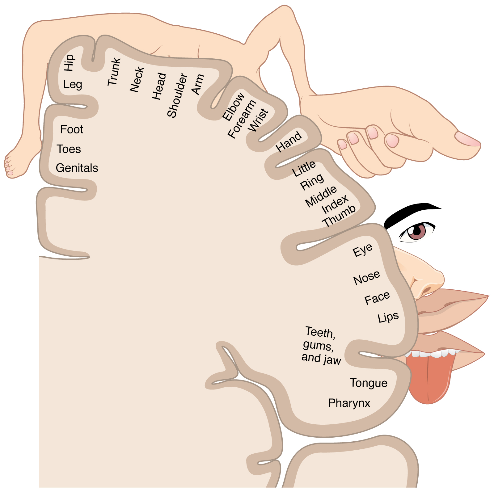
Spatial targets refer to the space targets, in order to produce specific sounds, our vocal tract needs to meet a specific spatial configuration. According to this model, there is an internal spatial representation of the vocal tract in the brain. It occurs in the Cortical homunculus close to the premotor cortex. (Has representations of different parts of the body [fig:homunculus]). In this area, there is more fine motor control and more motor firing than other regions(walking muscles, and other gross movements). According to these models, we move our Vocal Tract based on the initial configuration. We are making instantaneous changes of the spatial movements even in other configurations of the Vocal Tract (example: almost the same sound between /a/ with and without a pen in the mouth). The movement for a particular sound is not invariant, whereas speech perception is invariant.
Another type of targets is the Acoustic-auditory type. The goal is in the acoustic domain, to achieve what is being heard can also vary. So different articulatory movements can be achieved to produce a specific sound, and this will depend on the adjacent speech sounds, and the rate of speech. The hearing of the interlocutor is the target here.
Target models can be a combination of these two target outputs.
Connectionist models
These are models to study neural processing of the neural brain. One classic example under the umbrella of Connectionist model is the Parallel-distributed processing model or PDP. Even how complex our speech production model is, in order to keep up with the rate of speech, in order to convey the information we want to convey, the steps for speech production are not processed sequentially, but they are more or less in parallel.
1 or 2 co-articulators are triggered at the same time (or with small delay) to produce 2 different speech sounds that becomes co-articulation. There is a temporal meaning timing overlap. This models allows context sensitivity without increasing df.
- Extracted from [Wikiversity page of speech
- production](https://en.wikiversity.org/wiki/Psycholinguistics/Models_of_Speech_Production)
- “Dell’s model of spreading activation of lexical access is also commonly referred to as the Connectionist Model of speech production. Dell’s model claims, unlike the serial models of speech production, that speech is produced by a number of connected nodes representing distinct units of speech (i.e. phonemes, morphemes, syllables, concepts, etc.) that interact with one another in any direction, from the concept level (Semantic level), to the word level (Lexical selection level) and finally to the sound level (Phonological level) of representation. […] In contrast to serial models of speech production, Dell’s model can account for word blends, phrase blends, phonemic slips, and cognitive intrusions. This model explains these errors as the simultaneous activation of nodes that are either semantically or phonetically similar to the target.”
At inference time, a specific semantic word is activated through this network and will cascade the activations through a large interconnected weighted network, and the most activated will be chosen at each level [fig:dell].
This model addresses the several aspect of speech behaviours: serial order/co-articulation variability/do not increase degree of freedom.
![Dell’s Parallel-Distributed Processing
model[]{data-label="fig:dell"}](/images/dells_model.png) {width=”90.00000%”}
{width=”90.00000%”}
Speech Production models and language behaviour
So far all models deal with the speech production capacity, but the models are not embedded in the bigger picture of language production: prosody, rhythm is neglected… These models incorporate the segmental(phonemes, syllables) and suprasegmental aspects of speech.\
Neural models of speech production
These models identify the different part of the nervous systems that control various aspect of speech production. They identify the planning, programming, and execution roles of the different brain parts in speech production.
Review of “A Dynamical Approach to Gestural Patterning in Speech Production”
General concepts
Speech can be also portrayed a the process to arrange together a finite limited number of units to produce a very large well-formed utterances. Based on a finite set of phonemes which are discrete, static, and invariant across a variety of contexts, the individual forms words. This is the serial-order issue for speech production models. Yet, the observations of the produced speech is far from this hypothesis of discrete and context-free units. The focus of this paper is on the patterning of speech gestures, drawing on recent developments in experimental phonology/phonetics and in the study of coordinated behaviour patterns in multidegree-of-freedom dynamical systems. How to reconcile experimental observations of the acoustic and articulatory measures and the traditional linguistic analyses? The authors propose to answer this research question to study a dynamic model of articulation. In the paper, we have the following correspondences with “gestural units or primitives == degrees of freedom issue”, “articulatory consequence of partial or total temporal overlap of the activities of these gestural units (coproduction)==context-sensitivity issue” and “serial coupling among gestural primitives == Serial order issue”
[L]{}[0.5]{} 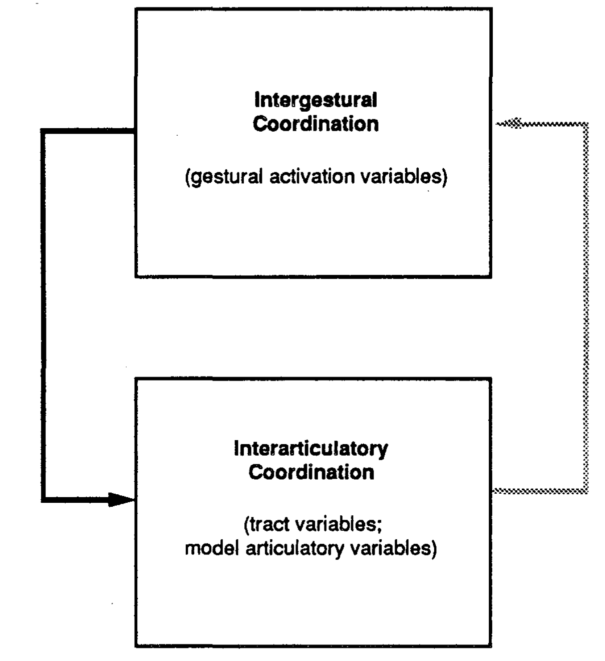 {width=”40.00000%”}
The main thesis of the paper is that speech emerge as behaviours implicit in a dynamical system with two functionally distinct but interacting levels. One level is the inter-gestural level, it corresponds to the set of activation coordinates; and there is the inter-articulator level which is defined for the articulator and tract variable coordinates. See figure [fig:dyn]
There is some evidence from experimental data that limbs and articulator movements is not hard wired controlled for muscles variables. These coordinative units must defined abstractly or functionally in a task-specific, flexible manner. These coordinative structures have been defined as task-specific and autonomous (time-invariant) dynamical systems that underlie an action’s form as well as its stability properties. The model is time-invariant for these task-domain sequence of abstract units.
During speech production, the articulators have to create and release constrictions locally in various regions of the vocal tract to produce the different sounds. In the task-dynamics models, the constrictions of the articulators are ruled by a dynamic system at the inter-articulator level see figure [fig:dyn].
One important distinction is : the tract variables are the system in which the context-independent gestural intents are framed, given. And the model articulators are the coordinates where context-dependent gestural intents/instructions are expressed. Each constriction type is associated with a pair of a pair of tract variables : the location along longitudinal axis of the vocal tract and the degree of constriction in the saggital plane. These constrictions/gestural types are mapped to a particular subset of model articulators. We will not make the detailed list of the constrictions measures (Lip aperture: vertical distance between the lips, lip protrusion: horizontal distance of the upper/lower lips to upper/lower teeth, etc.) and their corresponding articulatory constriction components. See figures 3 and 4 in [@saltzman1989dynamical].
Motion relationships between tract variables and articulators positions
For the simulations, we denote by $z$ the $m=9$ Vocal Tract variables. Each gesture in a simulated utterance is associated with a corresponding tract-variable dynamical system. Every variable is modelled as a damped second-order linear differential equation.
Here are the following tract-variable motion in equation [eq:motion]: \(\label{eq:motion} M \pdv[2]{z}{t} (t) + B \pdv{z}{t} (t) + K \Delta z(t) = 0\)
In [@deng1999computational], the vocal tract space dynamics equation is slightly different: a noise random component $w(t)$ is added, and there is a non-linear coefficients $S(t)$ for the damping and linear components.
\[\label{eq:ext_motion} \pdv[2]{z}{t} (t) + 2 S(t) \pdv{z}{t} (t) + S^2(t) \Delta z(t) = w(t)\]$z$ is a $\mathbb{K}{(m,1)}$ vector of current vocal tract variable positions. $\pdv{z}{t} ,\pdv[2]{z}{t} $ are the corresponding first and second order derivatives respect to time for $z$. We define $ \Delta z = z - z_0$ and $z_0\in \mathbb{K}{(m,1)}$ refers to the target or rest positions. $M \in \mathbb{K}{(m,m)}$ is the matrix of inertial coefficients, $B \in \mathbb{K}{(m,m)}$ is the matrix of damping coefficients.
These equations can be injected in the model articulator coordinates of the Haskins articulatory synthesizer. This synthesizer transforms the model articulator coordinates into the articulatory motion patterns. This transformation is about shape and size not mass, so it is a pure kinematic transformation.
Let’s dive in more details in these kinematic equations. A dynamical system for controlling the model articulators is specified by expressing tract variables $(z, \pdv{z}{t} , \pdv[2]{z}{t} )$ as functions of the corresponding model articulator variables $(\alpha, \pdv{\alpha}{t} , \pdv[2]{\alpha}{t} )$
\[\begin{aligned} z(t) &= z(\alpha(t))\\ \pdv{z}{t} (t) &= J(\alpha(t))\pdv{\alpha}{t} (t) \\ \pdv[2]{z}{t} (t) &= J(\alpha(t))\pdv[2]{\alpha}{t} (t) +\pdv{J}{t} (\alpha,\pdv{\alpha}{t})\pdv{\alpha}{t} (t)\end{aligned}\]$\alpha$ is a $\mathbb{K}{(n,1)}$ vector representing the current articulator positions. $z(\alpha(t)) \in \mathbb{K}{(m,1)} $ represents the tract variables expressed as a function of the current articulator positions. (The function $z$ should more properly defined).
$J(\alpha) \in \mathbb{K}{(m,n)}$ represents the *Jacobian Transformation Matrix* whose elements are defined as : $J{i,j} = \pdv{z_i}{\alpha_j} $. Therefore, a row in the Jacobian matrix represents the units of change for all tract variables according to one articulator variable $j$.
$\pdv{J}{t} (\alpha,\pdv{\alpha}{t}) \in \mathbb{K}_{(m,n)}$ results from differentiating each elements of $J$ with respect to time. Therefore, the elements of $\pdv{J}{t}$ are function of $\alpha$ and $\pdv{\alpha}{t}$.
The Jacobian and its derivative contains the geometric information and relationships between motions of the model articulators and the motions of the motions of the tract variables.
Using the equation of motion of $z$ from the Eq. [eq:motion], we derive the following equation for the articulator positions (We omit the variable $t$ for clarity):
\[\label{eq:art} M J(\alpha)\pdv[2]{\alpha}{t} + M \pdv{J}{t} (\alpha,\pdv{\alpha}{t})\pdv{\alpha}{t} + B J(\alpha)\pdv{\alpha}{t} + K \Delta z(\alpha) = 0\]We have still $\Delta z(\alpha) = z(\alpha(t)) - z_0$, and it is specified this variable should not be considered small.
So all admissible solutions $\Sigma$ for the model articulator variables need to respect this equation [eq:art].
At any time $t$, we can derive the Weighted pseudo inverse matrix $J^\star \in \mathbb{K}{(n,m)}$ of the Jacobian matrix $J$1 [@benati1980anthropomorphic]. It is defined by $J^\star = W^{-1}J^T(JW^{-1}J^T)^{-1}$ where $W \in \mathbb{K}{(n,n)}$ is a positive definite matrix that represents the articulatory weights. The pseudo inverse is used because there are more articulator variables than tract variables $n>m$. $J^\star$ gives us a unique, optimal least squares solution to the differential transformation from tract variables to the articulator variables.2
Using this relationship and as assumption that $M$ is invertible, we can obtain an articulatory acceleration vector $\alpha_A$ that represents the active driving forces during on the model articulators:
\[\label{eq:alphaart} \pdv[2]{\alpha_A}{t} = J^\star(M^{-1}[ - B J(\alpha)\pdv{\alpha}{t} - K \Delta z(\alpha) ]) - J^\star \pdv{J}{t}\pdv{\alpha}{t}\]Timings and Gestural activation variables
It is important different timing scales that captures that appear in the phenomenon of speech production: gestural duration or settling time and timing of activation of a gestural control unit.
The settling time for unperturbed discrete bilabial gesture is the time required for the system to move from an initial position with zero velocity to within a criterion percentage (e.g., 2%) of the distance between initial and target positions. Therefore a gesture’s settling time is determined by several factor which are the inertia, stiffness and damping parameters. These factors are intrinsic physical parameters of the associated tract-variable point attractor. This timing span is defined as the interaticulatory coordination level (bottom) of the task-dynamic model in figure [fig:dyn].
Another important timing is the span time of an activation of a gestural control unit. It is defined at the intergestural coordination (top) level of the task-dynamic model in figure [fig:dyn]. This is why it is introduced a third set of coordinates in addition of the tract variables and the articulators positions.
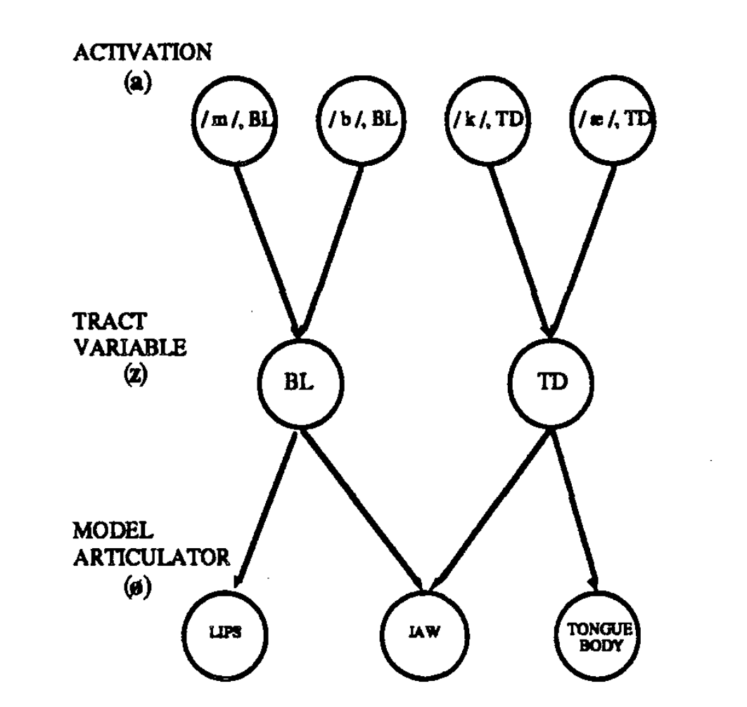
The third type of variables are the activation weights $a_{ik}(t)$ where $i$ represents the $i$-th tract variable and $k$ maps to the corresponding symbolic gesture’s linguistic unit ($k=/a/,/p/,/i/… $). These variables $a_{ik}(t)$ can be interpreted as the strength each symbolic gesture’s linguistic unit “attempts” to shape vocal tract movements at any given point in time $t$.
The three types are organised in three hierarchical levels [fig:var]. For notations clarity ø-variable from the paper is replaced with $\alpha$ in our document. Yet, there is no summation or any other constraint specified over a row or a column of activation at any time, just some set of values ${0,1}$ or boundaries $[0,1]$.
[L]{}[0.5]{}
 {width=”40.00000%”}
The temporal patterning of the gestural activity represents the activation of gestural primitives over time across parallel tract-variable output channels. For the simulations, a hand-made temporal sequence of activation of linguistic unit $A(t) = (a_{i,k}(t))\in \mathbb{K}{(m,p)}$ is generated with Haskins software based on a linguistic input. In the simulation, the $a{i,k}$ are normalised step-rectangular pulses but will be extended to continuous spectrum between 0 and 1.\
Coproduction
This part deals with the co-articulation or context-sensitivity phenomenon observed in the continuous realisation of speech. Several adjacent or near-adjacent segments can be measured or discerned in acoustic/articulatory measurements. Therefore, , these overlapping demands can be represented in the current modelisation as an overlapping/juxtaposition activation of patterns in a corresponding set of gestural scores.
First, how the gestural units have the control of the vocal tract? In the current schema, when a gesture activation ($/\Lambda/$ for instance) is at peak, this gesture has maximum of influence on the corresponding gesture’s tract-variable set. Between each gesture’s activation interval, the articulatory components are distributed according to the driving influences from the gestural level in the vocal tract space. When these activation units are minimals what is happening? This is called the Nonactive Gestural Control. We will treat as in the paper the active first, and the nonactive after.
These wave simulations are used for two main components: (1) Tuning the current set parameters of the equations $M,B,K,z_0$. (2) Gating the current pattern of tract-variable driving influences into the appropriate set of articulatory components.
There are two types of overlaps to distinguish: timing overlap and spatial overlap. Temporal overlap occurs when two or more activation gestures overlap in time. The spatial overlap occurs when ever two or more gestures that are time-overlapping share some or all of their articulatory components. The influence of timing and spatial overlapping is blended. This blending of time and spatial overlap is taking into account in the model as a function on how the matrix $A$ is injected in the interaticulatory dynamical system described before.
Parameter tuning
Each distinct gesture simulation is produced by a particular subset of tract variable and coordinate variables, and there is a corresponding set of time-invariant set of parameters linked to these coordinate systems.
(See the paper [@lammert2013statistical] for the parameter tuning problem done with statistical methods).